A13 – Photometric Stereo

In this activity, we would reconstruct a 3D object by using photometric stereo. An object is illuminated by the same point source with 4 different locations with respect to the object. The matlab file Photo.mat contains the 4 images corresponding to the 4 different locations.

According to the PDF file that Ma'am Jing sent us:
We can estimate the shape of the surface by capturing multiple images of the surface with the sources at different locations. The information about the surface will be coded in the shadings obtained from the images.
If there are N images in 3D space. We can define a matrix

where each row is a source, each column is the x,y,z component of the source. If we take N images of the surface using each of these N sources, then for each point (x,y) on the surface we have

Since I and V are already given we could compute for the matrix g by using the equation given below.

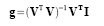
Then we get the normal vector by the equation below.

We can now calculate the shape of the object using the following equations.

We were given the matrix V.
V1 = {0.085832, 0.17365, 0.98106}
V2 = {0.085832, -0.17365, 0.98106}
V3 = {0.17365, 0, 0.98481}
V4 = {0.16318, -0.34202, 0.92542}

The data within the matlab file contains the intensity of the four images the intensities are in 128*128 matrices. We reshape these matrices into a row matrices in order to obtain the matrix I. Then when we finally get df/dx and df/dy by using the normal vector we reshape these back to a 128*128 matrices for us to reconstruct the 3D object. The four images below are the ones used in the activity. The following image is the reconstructed 3D object.

We see that the reconstructed 3D image is a sphere with a cross structure. This 3D image is similar to the 4 2D images which means that our reconstruction was successful.

I give myself a grade of 10 for successfully doing the activity.
Thank you for Rafael Jaculbia, Jorge Presto and Billy Narag for helping me in this activity. Also thanks to Cole and Jeric.

A12 – Correcting Geometric Distortions

This activity aims to correct geometric distortions which are a natural occurrence when taking pictures with a camera. The image below clearly shows a distorted image. We observe that the lines are not straight. What we aim here is to make the lines appear straight.

The instructions given can be summarized as follows:
1. Count the number of pixels down and across one box from the most undistorted grid of the image.
2. From the obtained data, we create an ideal and compute c1 to c8. We compute c1 to c8 by picking four points in the distorted image and then taking their respective coordinates in the ideal grid coordinate. Then using the equations below.

3. Per pixel in the ideal grid calculate the corresponding coordinate in the distorted grid. This can be done by using the equations below.

4. If the calculated coordinate is integer valued copy the grayscale value at that point onto the ideal grid pixel location. If the calculated coordinate is not integer valued then do interpolation by using the equation below.

I measured the size of a box with the most undistorted part of the image. The size was 9 pixels by 11 pixels. Then I created the ideal grid using scilab. The calculation of c1 to c8 were supposed to be per rectangle but it would take an eternity to do that so I picked a fairly large rectangle from the distorted image and took the coordinates of vertices and their corresponding coordinates in the ideal grid. Below is the table of the data that was recorded.

Ideal Coordinates		Real Coordinates
Xi	Yi	Xr	Yr
54	33	48	30
54	187	52	183
99	33	95	31
99	187	97	183

I calculated c1 to c8 and used it to know the corresponding location of each pixel in the ideal grid in the distorted grid. Then since it is more likely that the answer would be a non-integer I used interpolation. I did not use the round command since it is better to use the int command which gives the greatest integer value. I used this because I need the 4 nearest neighbors. For example if the coordinate was (9.5,10.6) I know that its nearest neighbors would be (9,10), (10,10), (9,11) and (10,11). If I used the round command it would be more difficult since I would have two cases which are round up or down so I used the int command. Using the int command the nearest neighbors of (x,y) would just be (int(x),int(y)), (int(x)+1,int(y)), (int(x),int(y)+1) and (int(x)+1,int(y)+1). The corrected image is shown below.

The resulting image is much less distorted than the original. We could improve the correction if we section the image and then calculate the corresponding c1 to c8 of each section which was the original instruction. Nevertheless, the correction was still successful and the interpolation was also done.

It took me quite a while to blog this activity so I give myself a grade of 8. Even though I was successful in doing the correction as well as the interpolation, I was still late. Sorry for the late posting but I did this activity on the day it was given. In fact I did it even though I was sick at that time laying in my bed with my laptop.

Thanks for everyone who helped me in this activity. Thank you Ma'am Jing because you chatted with me while I was sick. Thanks to Cole, Jeric and Julie. Special thanks for SPP and Bio 11 for preventing me to post this blog on time.

A11 – Camera Calibration

In this activity we try to calibrate our cameras. We do this by taking an image of a 3D calibration checkerboard. Then we assign a an origin and a right-handed coordinate system in the grid and measure around 20 to 25 corners of the squares of the checkerboard pattern. Each corner would have a coordinate [Xw, Yw , Zw]. From the image of the grid we get the coordinate [Yi, Zi] of each corners of the squares that we chose. These are the data that I have gathered:

Xw	Yw	Zw	Yi	Zi
0	0	0	100	36
1	0	2	90	72
1	0	4	90	112
0	1	5	117	131
0	3	7	154	168
0	4	4	171	106
0	3	2	152	69
0	6	1	205	44
0	5	8	191	185
4	0	7	57	164
5	0	4	46	100
4	0	1	58	42
2	0	9	80	208
7	0	2	23	52
6	0	8	35	181
0	7	6	228	142
0	4	10	173	227
5	0	10	47	225
0	2	9	137	208
0	5	2	188	65
0	6	5	209	123
6	0	6	35	139
0	6	10	211	225
3	0	5	69	125
7	0	11	24	244

Using these data we setup an appended matrix containing the some of the elements in the equation below.

The appended matrix of the leftmost matrix would be the matrix Q. The appended matrix of the rightmost matrix would be the matrix d. What we want to find is second matrix in the equation which we denote as matrix a. We do this by applying the equation below.

For my case I used excel to calculate and to construct the matrix but you could use other methods as well such as calculating it in scilab. I would not show the appended matrices but only the calculated matrix a.

Matrix a

-1.12E+01

16.47929

-3.72E-02

9.93E+01

-3.82E+00

-2.28E+00

1.88E+01

3.67E+01

-1.20E-02

-6.07E-03

-2.53E-03

1

Now we examine if these are correct. We use the equation

We use this to our previous data and try to see if we get the same [Yi, Zi] coordinates. The Table below shows the results and their difference from the known values.

Yr		Zr		Yi		Zi		delta Y		delta Z
99.26059921		36.6903502		100		36		0.739401		0.69035
89.53561712		71.7207949		90		72		0.464383		0.279205
89.92225298		110.57204		90		112		0.077747		1.42796
117.7563384		130.931302		117		131		0.756338		0.068698
153.9647225		167.560105		154		168		0.035278		0.439895
170.9055698		106.477688		171		106		0.09443		0.477688
152.1637482		69.0766455		152		69		0.163748		0.076645
206.1266372		43.4976498		205		44		1.126637		0.50235
191.0174924		185.15496		191		185		0.017492		0.15496
58.10852607		163.864721		57		164		1.108526		0.135279
46.48536116		99.8337782		46		100		0.485361		0.166222
57.41563756		42.3547116		58		42		0.584362		0.354712
80.32558877		208.104854		80		208		0.325589		0.104854
22.99597131		52.210583		23		52		0.004029		0.210583
35.14187397		180.953798		35		181		0.141874		0.046202
227.5075306		141.768338		228		142		0.492469		0.231662
173.3966707		226.951393		173		227		0.396671		0.048607
47.01195681		224.895651		47		225		0.011957		0.104349
136.650702		208.739956		137		208		0.349298		0.739956
188.2468657		65.2110463		188		65		0.246866		0.211046
208.1607909		123.1026		209		123		0.839209		0.1026
35.02876316		138.731433		35		139		0.028763		0.268567
210.7650967		225.019992		211		225		0.234903		0.019992
68.89331288		125.394012		69		125		0.106687		0.394012
23.20818217		244.182491		24		244		0.791818		0.182491
						Average		0.384953		0.297556

We see that there is little difference between the actual and the calculated values which means our calculated matrix a is approximately correct.

Now we use the calibration matrix a to predict the [Yi, Zi] coordinates of a known [Xw, Yw, Zw] coordinates then we compare it to the actual values. The results are below.

Xw	Yw	Zw			Yr		Zr		Yi		Zi		0.384953
7	0	10			23.18406822		222.368334		23		222		0.184068
0	0	11			101.6775298		250.622298		102		250		0.32247
0	8	0			242.8889262		19.3613035		242		19		0.888926
0	7	3			225.8096953		81.2166586		226		81		0.190305
0	6	7			209.1941664		163.542911		209		163		0.194166
0	7	11			230.3987701		244.881633		230		245		0.39877
											Average		0.363118

We see that our predictions correspond fairly well with our actual values. This further verifies that our calculated matrix a is correct. The image below is the grid and the blue dots are the points used to find the calibration matrix and the block dots are the points whose [Yi, Zi] coordinates were determined using the calibration matrix.

I give myself a grade of 10 for this activity since I have successfully calculated the calibration matrix and also verified its validity by predicting values for a set of real world coordinates.
Thank you for Jorge Presto and Billy Narag for collaborating with me in this activity.

A10 – Preprocessing Handwritten Text

In this activity we would use all that we have learned to preprocess handwritten text. We would choose from the two images that was given and then crop a portion of it that we would like to process. The image that I chose is shown below as well as the portion I want to work on. I chose that portion since it has the most number of text and it seems that the handwriting is fine.




We need to remove the lines that are present in order for us to see only the text. From the previous activities, we do this by making a filter in the frequency domain and blocking the frequencies corresponding to this lines. From previous activities we know the horizontal lines correspond to a vertical line at the center in the frequency domain. We check this by looking at the Fourier transform of the image. The FT and the mask created is shown below.



The resulting image is shown below.




The lines are already removed enough for the text to be isolated. Now we need to binarize the image. We do this by looking at its histogram and getting the threshold. I have done this and also inverted the colors since the background should be black and the text should be white for us to use morphological operations in scilab. The resulting image is shown below.



The letters are still readable in this case. We just need to close the gaps that the lines have made and also to make the text only one pixel in thickness. We do this by using the close operation. I use a 2*1 structuring element in this case. I also eroded it by the a same structuring element for the letters to thin out. The resulting image is shown below.



The lines are already removed and also the handwriting can still be recognized like the VGA Cable and the 2 Cable text below. I rate myself 10 out of 10 for this activity since I have successfully done the task and have applied what I learned in the previous activities. I have done this at home since I could not come to class.

A9 – Binary Operations

In this activity we want to estimate the area of one "cell" in the image that was given. A circle corresponds to one cell. What we want to do is to find the areas of all the circles then average them to get the approximate area of one circle. We do this by pixel counting following the procedure below.

1. Cut the given image to 256*256 sub-images. Save in filenames with increasing
index number, e.g. C1_01.jpg, C1_02.jpg etc.
2.Find it's thresholding value to separate the cells from the background.
3.Binarize the sub-images according to the threshold value using command imb2w.
4.Do opening and closing operations on the sub-images to clean the image (removing the isolated pixels, separating connected blobs and filling out holes). Opening operation is an erosion of an image followed by a dilation using the same structuring element. Closing is a dilation of an image followed by an erosion using the same structuring element.
4. Use bwlabel to label each contiguous blob on the binarized sub-images.
5. Find the areas of each blob by pixel counting and then find the estimate of the "cell" area using these values.

The image that I used is shown below as well as one of its sub-image.




What I did was to first close the image using a 10 pixel radius circle then open it using the same circle. The result for the figure above is shown below.



This is already a good image since it looks clean and there are no stray pixels. Although some of the blobs are still overlapping each other. We did this to all the sub-images and got the areas in each sub-images. This would be tiresome to do for 9 sub-images so I designed my program to do this automatically for each index. I plotted the histogram of the areas.



It looked like the areas are clustered between 400 and 600 so I looked more closely at that area and zoomed in. The image below is the histogram between 400 and 600.


Looking carefully the correct range that should be considered must be from 480 to 580. So I took the average of the areas that fall between those values and get the standard deviation. The values calculated were area = 537.42857 and standard deviation = 18.544518. This is a fairly good estimate since the standard deviation is much smaller than the mean which means that the considered values are not that far from the real value of the area.

Thank you for Julie Mae Dado, Marge Maallo (Happy Birthday), Cole Fabros, Rafael Jaculbia, Eduardo David, Jorge Presto and Billy Narag for their help.

I rate myself 10 out of 10 since I have successfully estimated the value of the are for each blob and I think that I have done what is necessary to estimate it accurately. Also, I have figured out a way to process the sub-images automatically without running them one by one.
The code is shown below:

function [bin, recurrence] = histogram(image_matrix)
imsize = size(image_matrix)
bin = matrix(0:(max(image_matrix)),[(max(image_matrix)+1),1]);
recurrence = bin.*0;
for i = 1:imsize(1)
for j = 1:imsize(2)
recurrence(image_matrix(i, j) + 1) = recurrence(image_matrix(i, j) + 1) + 1;
end
end
endfunction

chdir('C:\Documents and Settings\Abraham\My Documents\AP186\A9');
counter=1;
area=[]
j=1;
for j= 1:9
a="c1_0"+string(j)+".jpg"; //opening each filename automatically
i=imread(a);
im=im2bw(i,.8);
e=imread('e.bmp');
r=dilate(im,e); //closing operation
r=erode(r,e);
r=erode(im,e); //opening operation
r=dilate(r,e);
[b,n]=bwlabel(r);
[x,y]=histogram(b);
x=x(2:max(b+1));
y=y(2:max(b+1));
g=1;
for k=counter:counter+n-1
area(k)=y(g);
g=g+1;
end
counter=counter+n;
end

scf(1);
histplot(length(area),area);

x=find(area<600>480);
scf(2)
histplot(length(x), area(x));
a=area(x);

a=sum(a)/length(x) //area
y=stdev(area(x)) //error

A8 – Morphological Operations

In this activity we tried to predict the effect of dilation and erosion operations on some shapes using different structuring elements. Dilation's effect is to expand the object in the shape of the structuring element. Erosion's effect is to reduce the object by the shape of the structuring element. The shapes that were dilated and eroded were a binary image of a square (50×50) , a triangle (base = 50 , height= 30), a circle (radius 25), a hollow square (60×60, edges are 4 pixels

thick), and a plus sign (8 pixels thick and 50 pixels long for each line). The structuring elements used were 4×4 ones, 4×2 ones, 2×4 ones, cross (5 pixels long, one pixel thick). We have drawn our prediction of what would be the shape in a yellow pad. Then we verified it using the function dilate and erode in scilab.

The first image is the original image followed by the dilated and eroded images using the structuring elements (4×4 ones, 4×2 ones, 2×4 ones, cross).

Square (Dilated)

Square (Eroded)

Triangle (Dilated)

Triangle (Eroded)

Circle (Dilated)

Circle (Eroded)

Hollow Square (Dilated)

Hollow Square (Eroded)

Cross (Dilated)

Cross(Eroded)

My predicted shapes were verified using the scilab. My predictions were correct except for the cross eroded by a cross. I did not expect that square structure on the center. I expected it to be also a cross. Nevertheless, I rate myself 10 out of 10 for successfully completing the task given. It took me a lot of time to draw and predict but it was quite fun. Thank you for Ma'am Jing for personally helping me. Also thanks for Billy Narag and Jorge Michael Presto for collaborating with me.

A7 – Enhancement in the Frequency Domain

Anamorphic property of the Fourier Transform

We created a 2D sinusoid using scilab then we took its Fourier Transform and displayed the FT modulus. The images below are the 2D sinusoid(right) and its FT (left). The frequency of the sinusoid is 4.


We see that the sinusoid is propagating in the horizontal axis. The FT image has two dots in the horizontal axis. We can consider only one dot because we know that the FT gives a mirror image of the frequencies. In the FT of a 1D sinusoid, we see that if you increase the frequency of the sinusoid then the peak would be seen farther in the axis. We checked if this is also the case for a 2D sinusoid. It seems that this was also the case since we saw that the dots are farther away for the origin(center of image) which means that the peak is farther from the axis. The images below are the sinusoids(left) and their FTs(right).

Frequency = 8

Frequency = 16

We also checked the effect of rotation of the sinusoid to its FT. We observed that the rotation of the sinusoid also rotates its FT. Below are the images of the rotated sinusoids(left) and their FTs(right). It seems that the rotation in the vertical axis in the spatial domain causes a rotation in the horizontal axis in the frequency domain as seen below.

theta = 30

theta = 45

theta = 60

We also tried a combination of sinusoids. The resulting image and its FT is shown below. For a combination of sinusoids, one in the x axis and one in the y axis, the FT has 4 dots which are in different quadrants. This represents the product of the supposedly 2 dots in the x axis and 2 dots in the y axis.



Fingerprints : Ridge Enhancement

We opened an image of a finger print as a grayscale image in scilab. We get the FT to find where the frequencies of the ridges lie. Using the mkfftfilter command in scilab we make a high-pass filter which allows only the frequencies that we specify. We then get the convolved image of the filter and the finger print. Below are the image of the FT of the finger print as well as of the mask. We can use the log function to show all the frequencies that are present if they are not visible.


The images below are the fingerprint(left) and the enhanced image(right) using the filter. The filter used is a high-pass filter which lets the components with high frequencies pass through and discards the low frequency components. We can see that the fingerprint image is greatly improved.



The finger print is from the site
http://www.dailymail.co.uk/news/article-518628/Foreigners-thrown-Britain-refuse-details-ID-cards.html

Lunar Landing Scanned Pictures : Line removal

In this part of the activity we attempt to remove the line in the lunar landing scanned picture below.

In the first part of our activity we noticed that horizontal lines appear to be dots in the vertical axis of our FT. We take the FT of this image and see if we can compare it to what we have seen in the first part of the activity. We expect to see dots or lines in the horizontal axis of our FT since we have vertical lines in our image. Below is the FT of the image.

We see that there are indeed dots and a line in the horizontal axis. We could interpret this as the line that we see in the spatial domain. We prepare a mask that would filter out this dots and line in the frequency domain in the same way retaining the other vital information. The filter looks like this.

The resulting image using this filter is shown below.

We see that our image is now free of the line that we see before but there are some information that were also erased. We could not exactly point out where the frequency of that vertical line lie in the frequency domain. Still, we have enough information to some extent to show the lunar picture quite nicely. 

Thanks for Cole Fabros for lots of help. Thanks also for Rafael Jaculbia and Jorge Michael Presto.

I rate myself 10 since I have successfully finished the activity and have done what was required. Also, I have gained quite an understanding of FTs although I believe I still need more practice and learning to do.