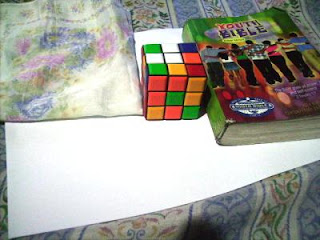
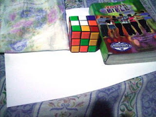
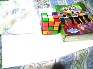
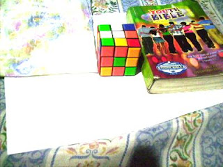
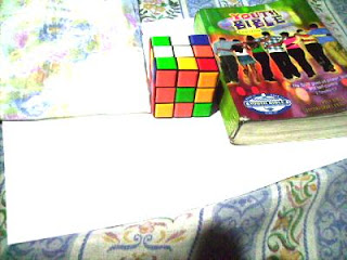
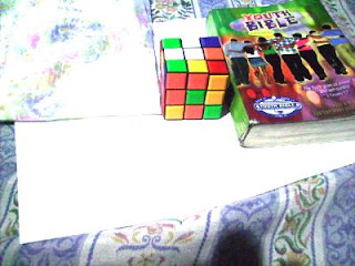
In this activity we invoke two well-known white balancing algorithms, the Reference White Algorithm (RW) and the Gray World Algorithm (GW). The first part is to examine different kinds of white balancing and their images. I took pictures of the same object using different white balancing settings. The object that I used were a rubix cube, a green Bible and a handkerchief. The objects were placed on top of a bond paper which is our white reference. The images are shown below.


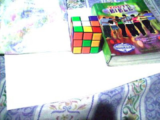
Auto WB and Cloudy WB


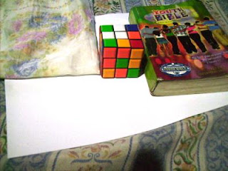
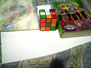
Daylight WB and Flourescent WB

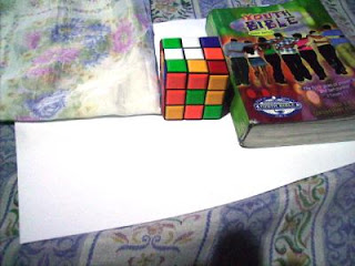
Tungsten WB
We could see that not all WB have satisfactory accuracy in the image color. This is obvious because the bond paper that was supposed to be white appears to be colored. That is why we use the white balancing algorithm discussed. The first would be the RW algorithm. We take the RGB value of the white reference and call the values Rw, Gw and Bw. Then for each pixels of the image we divide Rw, Gw, and Bw to the corresponding values (R value divided by Rw, G by Gw and B by Bw). If there are values that exceed 1 then we change that value to 1. The resulting images are shown below.
Previously Auto WB and Cloudy WB
Previously Daylight WB and Flourescent WB
Previously Tungsten WB


Previously Auto WB and Cloudy WB


Previously Daylight WB and Flourescent WB

Previously Tungsten WB
We can observe that all our images are greatly improved using the RW algorithm. Also, it seems that the images are almost identical. This may be due to the fact that different white balancing in cameras are in fact just multiplying certain RGB coefficients to the corresponding RGB values of the image. This means that if we divide it by those RGB coefficients we get the original pixel value that the camera measured (original meaning unprocessed or no white balancing). That is just what we did when we divided the RGB value of the white reference. That is why we just ended up having the original image that the camera captured.
Now we try using the GW algorithm. The concept is the same as in the RW algorithm. The only difference is the RGB values of the white reference is the mean of the RGB values of the image. We get Rw by getting the mean of the R values of the image. This is the same for Gw and Bw. The resulting images using the GW algorithm are shown below.
Previously Auto WB and Cloudy WB
Previously Daylight WB and Flourescent WB
Previously Tungsten WB
Now we try using the GW algorithm. The concept is the same as in the RW algorithm. The only difference is the RGB values of the white reference is the mean of the RGB values of the image. We get Rw by getting the mean of the R values of the image. This is the same for Gw and Bw. The resulting images using the GW algorithm are shown below.


Previously Auto WB and Cloudy WB


Previously Daylight WB and Flourescent WB

Previously Tungsten WB
The images are still greatly improved compared to the original image. It seems that the images are almost the same. This may have the same explanation as in the RW algorithm. At this stage I cannot determine which is better. It seems that both algorithm have promising results. We proceed further by taking a picture of objects of the same hue using the wrong white balancing setting. Then we perform both the RW and GW algorithm on the image. The image is shown below as well as the resulting image using RW algorithm and the resulting image using GW algorithm.
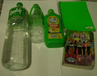
Original Image
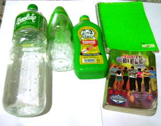
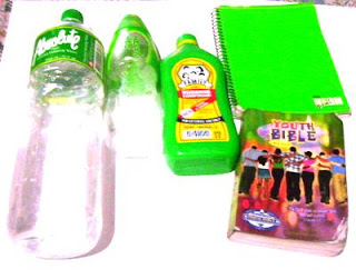
Image using RW algorithm and GW algorithm

Original Image


Image using RW algorithm and GW algorithm
Both images are better than the original image. I think that the image using RW algorithm is better in this case. The image using GW algorithm seems very bright and has poor contrast. This may be because the reference of for the GW algorithm is dependent on which RGB values are prominent in the image. This is due to the fact that the GW algorithm uses the mean of the RGB values of the image. For example if the color dominant in the image is green then the reference would be closer to the RGB values of the green. When we apply the GW algorithm on that image the green would appear closer to white. This explains why our image using the GW algorithm appeared brighter. If all the major hues are represented in the image then I think the GW algorithm would have better results since the average of the RGB values would most likely represent the average color of the world which is assumed to be gray.
I give myself a grade of 10 for this activity since I have done the algorithms and also included possible explanations for the results. Thank you for Billy Narag for helping me in this activity.
I give myself a grade of 10 for this activity since I have done the algorithms and also included possible explanations for the results. Thank you for Billy Narag for helping me in this activity.


