This activity is similar to the last two activities in which we try to identify what class an object belongs to. This time we are going to use neural networks which compose of three parts. These are the input layer, hidden layer and the output layer. The input layer contains the characteristics in which the objects can be distinguished and the output layer would tell which class the object belongs to. I would use the same classes I used in activity 19. The two classes are the quail eggs and the squid balls. Neural networks needs to train themselves with the objects and their classification in order to be more efficient in classifying the objects later on. The code was given by Jeric. The modified code is given below for my data set. The code is shown below.
--------------------------------------------------------------------------------------------------
// Simple NN that learns 'and' logic
// ensure the same starting point each time
rand('seed',0);
// network def.
// - neurons per layer, including input
//3 neurons in the input layer, 8 in the hidden layer and 1 in the ouput layer
N = [3,8,1];
// inputs
x = train = fscanfMat("train.txt")';// Training Set
// targets, 0 if squidballs, 1 if quail eggs
t = [0 0 0 0 1 1 1 1 ];
// learning rate is 4 and 0 is the threshold for the error tolerated by the network
lp = [4,0];
W = ann_FF_init(N);
// 1000 training cyles
T = 1000;
W = ann_FF_Std_online(x,t,N,W,lp,T);
//x is the training t is the output W is the initialized weights,
//N is the NN architecture, lp is the learning rate and T is the number of iterations
// full run
j=ann_FF_run(x,N,W) //the network N was tested using x as the test set, and W as the weights of the connections
--------------------------------------------------------------------------------------------------
The results were
[5.34E-03 7.41E-02 1.44E-02 8.34E-03 0.99132471 0.952957436 0.97008475 0.981131133]
Rounding off shows a 100% accuracy. The weakness of this method is it needs to train first a lot of times and also needs a number of samples in order to distinguish between classes. Our brain is far more advance since we can automatically tell which is which even if we just saw it once.
I give myself a grade of 10 in this activity since I was able to understand and employ neural networks in classifying objects. Thank you for Jeric for the code.
Sunday, October 12, 2008
Saturday, October 4, 2008
A19 – Probabilistic Classification
In this activity we try to classify objects into classes using Linear Discriminant Analysis (LDA). A detailed discussion was given by Dr. Sheila Marcos in the pdf file given by Dr. Maricor Soriano.


We used two classes from the previous activity. I used the quail eggs class and the squid balls class. I already obtained its features from the previous activity. The features I chose were the mean of normalized r and g value as well as the product of their standard deviation. The features are shown below for the two classes.

Using this set of data I calculated the covariance matrix in scilab using the process described in the pdf file. The covariance matrix calculated is shown below.

Then using this covariance matrix we calculate for the discriminant values using scilab. The results are shown below.

Then using this covariance matrix we calculate for the discriminant values using scilab. The results are shown below.

We see that the classification was 100% accurate which means the we were successful in employin LDA to our given data.
I give myself a grade of 10 for this activity since I have achieved a good result using LDA. No one helped me in this activity. I think this is one of the easiest activity.
chdir('D:\Mer\Documents\Majors\AP186\A19\');
vector=[];
for j=1:8
img = imread("k"+string(j)+".jpg");
i = (img(:, :, 1) + img(:, :, 2) + img(:, :, 3));
r = img(:, :, 1)./i;
g = img(:, :, 2)./i;
b = img(:, :, 3)./i;
mnr=mean(r);
mng=mean(g);
str=stdev(r);
stg=stdev(g);
strg=str*stg;
k(j,:)=[mnr,mng,strg];
end
uk=[mean(k(:,1)),mean(k(:,2)),mean(k(:,3))];
for j=1:8
img = imread("sq"+string(j)+".jpg");
i = (img(:, :, 1) + img(:, :, 2) + img(:, :, 3));
r = img(:, :, 1)./i;
g = img(:, :, 2)./i;
b = img(:, :, 3)./i;
mnr=mean(r);
mng=mean(g);
str=stdev(r);
stg=stdev(g);
strg=str*stg;
s(j,:)=[mnr,mng,strg];
end
us=[mean(s(:,1)),mean(s(:,2)),mean(s(:,3))];
u=uk*8+us*8;
u=u/16;
xk=[];
xs=[];
for j=1:8
xk(j,:)=k(j,:)-u;
xs(j,:)=s(j,:)-u;
end
ck=(xk'*xk)/8;
cs=(xs'*xs)/8;
C=.5*(ck+cs);
Ci=inv(C);
kk=uk*Ci*k'-0.5*uk*Ci*uk'+log(0.5);
ks=us*Ci*k'-0.5*us*Ci*us'+log(0.5);
sk=uk*Ci*s'-0.5*uk*Ci*uk'+log(0.5);
ss=us*Ci*s'-0.5*us*Ci*us'+log(0.5);
Monday, September 15, 2008
A18 – Pattern Recognition
It fascinating for the human brain to classify objects by just seeing them even though what they see includes a lot of information such as color, size, smoothness, etc. We might not have realized it but we could classify objects almost instantaneously and make decisions based on what we see. Computers, however, takes time in order to do such things and are not perfect.
In this activity we would try to classify a set of images using the minimum distance classification.
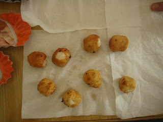
Let wj where j = 1, 2, 3 ... W be a set of classes and W the total number of classes. If we define a representative of class wj to be its mean feature vector then


In this activity we would try to classify a set of images using the minimum distance classification.
Let wj where j = 1, 2, 3 ... W be a set of classes and W the total number of classes. If we define a representative of class wj to be its mean feature vector then

where xj is the set of ALL feature vectors in class wj and Nj is the number of samples in class wj. The simplest way of determining class membership is to classify an unknown feature vector x to the class whose mean or representative it is nearest to. For example, we can use the Euclidean distance


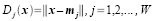
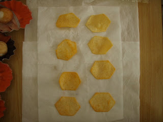
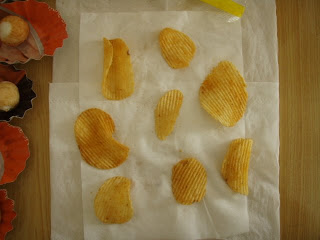
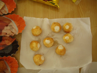
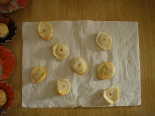
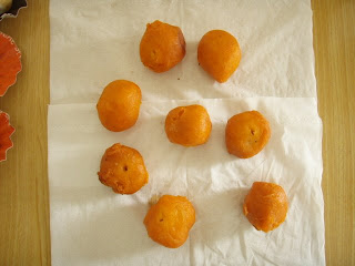
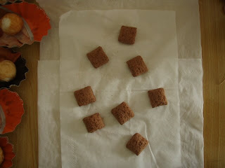
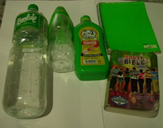
The objects I tried to sort out are the foods we bought near the math building. These are quail eggs, squid balls, chicken balls, fish balls, v-cut, piatos, and pillows. (We almost ate it while we were on the way back to CSRC.lol) We took images of each of these foods by their class then obtained their feature vector. The feature vector I used contained the mean chromaticity values r and g of the class as well as the mean of the standard deviation of its chromaticity. I believe these are the information that would most distinguish each class from one another. The images are shown below (drools....)


I tried to classify 21 samples using the minimum distance classification method and got the follow results
The accuracy of classification is 90%. This is quite good. This means the classifiers we used are indeed the relevant information.
I give myself a grade of 10 out of 10 for this activity for having classified samples with a fairly high accuracy. I thank Raf, Jorge, Ed and Billy for helping me in this activity. Special thanks to Cole, JC and Benj for the food.^_^
| Predicted | ||||||||||
| quail eggs | squid balls | chicken balls | fish balls | piatos | v-cut | pillows | ||||
| Actual | quail eggs | 3 | ||||||||
| squid balls | 3 | |||||||||
| chicken balls | 3 | |||||||||
| fish balls | 3 | |||||||||
| piatos | 3 | |||||||||
| v-cut | 1 | 1 | 1 | |||||||
| pillows | 3 | |||||||||
The accuracy of classification is 90%. This is quite good. This means the classifiers we used are indeed the relevant information.
I give myself a grade of 10 out of 10 for this activity for having classified samples with a fairly high accuracy. I thank Raf, Jorge, Ed and Billy for helping me in this activity. Special thanks to Cole, JC and Benj for the food.^_^
Wednesday, September 10, 2008
A17 – Basic Video Processing

For this activity, we are tasked to apply what we learned in order to extract essential data from a video of a kinematic process. The video that I processed is that of a solid cylinder rolling along the incline (without slipping). In order to do this we decomposed the video into several images corresponding to each of its frames. We did this by using the software Virtual Dub. I used two techniques in order to get the position of the cylinder. First is image segmentation where I segmented by parametrically. Since the output is not in the range of 0-255 which is the range of grayscale values, I applied histogram stretching which I learned in the activity involving histogram manipulation. Then I applied thresholding to clear off everything except for the cylinder. The binarized video is shown below.
I plotted the position of the centroid of the cylinder versus time and then fitted a 2nd order polynomial trendline and obtained it's equation. The coefficient of the 2nd order term is just half the acceleration of the centroid since the acceleration is just the double derivative of the position with respect to time. The plot is shown below.

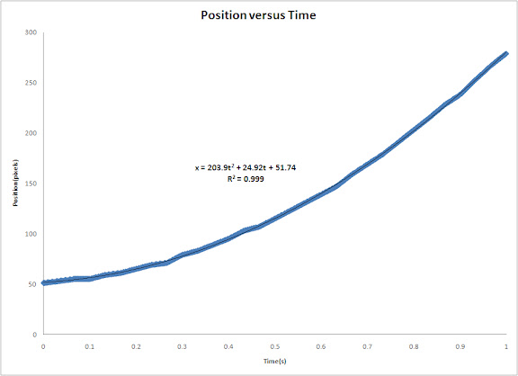
The acceleration using the equation of the trendline is 407.8 pixels/s^2. pixel to mm ratio is 1pixel : 1.5mm. Converting the acceleration to m/s^2, we get 0.6117 m/s^2. The code I used is shown below.
img = imread("a.jpg");
II = (img(:, :, 1) + img(:, :, 2) + img(:, :, 3));
r = img(:, :, 1)./II;
g = img(:, :, 2)./II;
b = img(:, :, 3)./II;
cen=[];
for ii=0:31
img1 = imread(string(ii)+".jpg");
I = (img1(:, :, 1) + img1(:, :, 2) + img1(:, :, 3));
R = img1(:, :, 1)./I;
G = img1(:, :, 2)./I;
B = img1(:, :, 3)./I;
//Parametric Segmentation
mnr=mean(r);
mng=mean(g);
str=stdev(r);
stg=stdev(g);
pr=1/(str*sqrt(2*%pi));
pr=pr*exp(-(R-mnr).^2/2*str);
pg=1/(stg*sqrt(2*%pi));
pg=pg*exp(-(G-mng).^2/2*stg);
P=pr.*pg;
//Histogram Stretching
imcon=[];
con=linspace(min(P),max(P),256);
for i=1:size(P,1)
for j=1:size(P,2)
dif=abs(con-P(i,j));
imcon(i,j)=find(dif==min(dif))-1;
end
end
P=imcon;
T=im2bw(P,.9);
[y,x]=find(T==max(T));
cen(ii+1)=(max(x)+min(x))/2;
imwrite(T,"new"+string(ii)+".jpg");
end
//Interpolation of position versus time
x=0:1/30:31/30;
xx=linspace(0,31/30,1000);
yy=interp1(x,cen,xx)
write("position.txt",yy');
write("time.txt",xx');
The other technique I uses was by just simply thresholding the grayscale images. I applied thresholding the grayscale images and then used a couple of closing and opening operations to remove unwanted parts. The resulting binarized video is shown below.
Again, I plotted position of the centroid of the cylinder versus time and get the trendline and equation to find the acceleration. The plot is shown below.
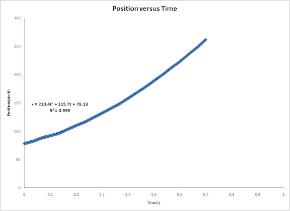
The acceleration using the equation of the trendline is 420.8 pixels/s^2. pixel to mm ratio is 1pixel : 1.5mm. Converting the acceleration to m/s^2, we get 0.6312 m/s^2. The code I used is shown below.
for i=0:21
im=imread(string(i)+".jpg");
im=im2bw(im,.74);
se=ones(4,10);
im=dilate(im,se);
im=erode(im,se);
se=ones(4,7);
im=erode(im,se);
im=dilate(im,se);
[y,x]=find(im==max(im));
cen(i+1)=max(x);
imwrite(im,"new"+string(i)+".jpg");
end
//Interpolation of position versus time
x=0:1/30:21/30;
xx=linspace(0,21/30,1000);
yy=interp1(x,cen,xx)
write("position.txt",yy');
write("time.txt",xx');
We need to verify if our calculated values are close to the theoretical value. I relived my Physics 101 days and solved the equation. The solution is shown in the link below (just click the pic).
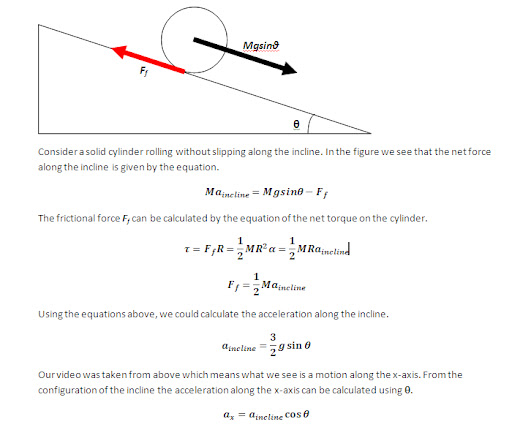
The calculated theoretical acceleration is 0.6345 m/s^2. For the parametric segmentation technique the error was 3% while for the thresholding technique the error was 0.5%. Both have fairly low errors. This means that our video processing was successful.
I rate myself a 10 out of 10 (even more) for finishing this activity and showing two techniques to achieve what was required. Thank you for Raf, Ed, Jorge and Billy for helping in this activity and helping me process the video and also create a gif animation. I really enjoyed it.
for i=0:21
im=imread(string(i)+".jpg");
im=im2bw(im,.74);
se=ones(4,10);
im=dilate(im,se);
im=erode(im,se);
se=ones(4,7);
im=erode(im,se);
im=dilate(im,se);
[y,x]=find(im==max(im));
cen(i+1)=max(x);
imwrite(im,"new"+string(i)+".jpg");
end
//Interpolation of position versus time
x=0:1/30:21/30;
xx=linspace(0,21/30,1000);
yy=interp1(x,cen,xx)
write("position.txt",yy');
write("time.txt",xx');
We need to verify if our calculated values are close to the theoretical value. I relived my Physics 101 days and solved the equation. The solution is shown in the link below (just click the pic).
The calculated theoretical acceleration is 0.6345 m/s^2. For the parametric segmentation technique the error was 3% while for the thresholding technique the error was 0.5%. Both have fairly low errors. This means that our video processing was successful.
I rate myself a 10 out of 10 (even more) for finishing this activity and showing two techniques to achieve what was required. Thank you for Raf, Ed, Jorge and Billy for helping in this activity and helping me process the video and also create a gif animation. I really enjoyed it.
Wednesday, September 3, 2008
A16 – Color Image Segmentation


In this activity we do image segmentation using the normalized chromaticity coordinates(NCC) of each pixel of the region of interest(ROI) of an image using their RGB values. The image and the ROI is shown above.

Since b is just 1-r-g, it is sufficient to only know the r and g values. In this way we simplify our work since we would only deal with those two values.
The first segmentation technique we used is the probability distribution estimation or the parametric segmentation. We first calculated the mean and the standard deviation of the r values of the ROI. After this, we go to the image we want to segment and then calculate the probability of each pixel having a chromaticity r to belong to the ROI by using the gaussian probability distribution given by the equation below.
The first segmentation technique we used is the probability distribution estimation or the parametric segmentation. We first calculated the mean and the standard deviation of the r values of the ROI. After this, we go to the image we want to segment and then calculate the probability of each pixel having a chromaticity r to belong to the ROI by using the gaussian probability distribution given by the equation below.


As we can see the image was segmented. The bright region is the segmented region. The darker region is the unsegmented region.
The second technique we used was histogram back projection. We first get the 2 dimensional histogram of the ROI based on its r and g values. Since both the r and g values ranges from 0 to 1 I divided it to 256 divisions which means there are 256 values in the both the r and g axis of the 2d histogram ranging from 0 to 255. The histogram is shown below.

After we get the histogram of the ROI we normalize it. For each pixel in the image we want to segment we find its r and g values and then locate it's normalized histogram value. The histogram value would now be the value of the pixel of the segmented image. The segmented image is shown below.

We see that the segmentation seems to be similar to the parametric segmentation. It is obvious that only the segment with the closest chromaticity of the ROI can be seen.
The two techniques are both good at segmenting the image. The parametric segmentation was used assuming a normal distribution but it may not always be the case. The back projection method was much faster since no further calculations of the probability distributions were needed. In this activity I think the results of the parametric segmentation was better. Using the back projection method woult make pixels which are not of the patch. equal to zero. If there were some slight variations it would not belong to be segmented anymore even if it seems to be of the same chromaticity. The parametric segmetation was based on probability so even if there were slight variations it would still be segmented as long as it is close to the chromaticity of the patch. This may explain why the parametric segmentation appears brighter and some regions are not totally dark.
I give myself a grade of 10 for this activity since I have both implemented the techniques and also seem to give a reasonable explanation of the results. Comments would be highly encourage since I want to verify if my explanations were correct.
Thank you for Ma'am Jing, Jorge, Rap, Ed and Billy for helping in this activity.
Thursday, August 28, 2008
A15 – Color Image Processing
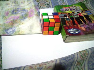
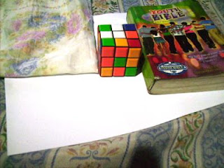
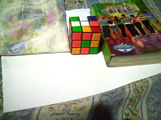
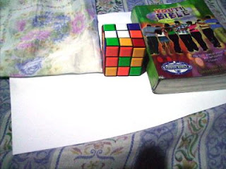
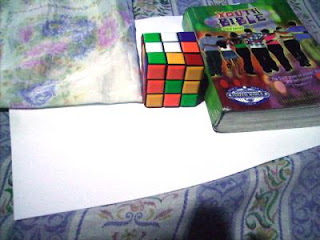
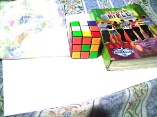
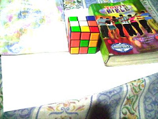
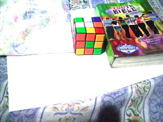
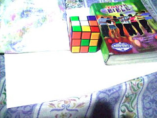
In this activity we invoke two well-known white balancing algorithms, the Reference White Algorithm (RW) and the Gray World Algorithm (GW). The first part is to examine different kinds of white balancing and their images. I took pictures of the same object using different white balancing settings. The object that I used were a rubix cube, a green Bible and a handkerchief. The objects were placed on top of a bond paper which is our white reference. The images are shown below.


Auto WB and Cloudy WB


Daylight WB and Flourescent WB

Tungsten WB
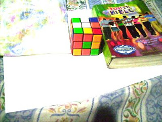
We could see that not all WB have satisfactory accuracy in the image color. This is obvious because the bond paper that was supposed to be white appears to be colored. That is why we use the white balancing algorithm discussed. The first would be the RW algorithm. We take the RGB value of the white reference and call the values Rw, Gw and Bw. Then for each pixels of the image we divide Rw, Gw, and Bw to the corresponding values (R value divided by Rw, G by Gw and B by Bw). If there are values that exceed 1 then we change that value to 1. The resulting images are shown below.
Previously Auto WB and Cloudy WB
Previously Daylight WB and Flourescent WB
Previously Tungsten WB


Previously Auto WB and Cloudy WB


Previously Daylight WB and Flourescent WB

Previously Tungsten WB
We can observe that all our images are greatly improved using the RW algorithm. Also, it seems that the images are almost identical. This may be due to the fact that different white balancing in cameras are in fact just multiplying certain RGB coefficients to the corresponding RGB values of the image. This means that if we divide it by those RGB coefficients we get the original pixel value that the camera measured (original meaning unprocessed or no white balancing). That is just what we did when we divided the RGB value of the white reference. That is why we just ended up having the original image that the camera captured.
Now we try using the GW algorithm. The concept is the same as in the RW algorithm. The only difference is the RGB values of the white reference is the mean of the RGB values of the image. We get Rw by getting the mean of the R values of the image. This is the same for Gw and Bw. The resulting images using the GW algorithm are shown below.
Previously Auto WB and Cloudy WB
Previously Daylight WB and Flourescent WB
Previously Tungsten WB
Now we try using the GW algorithm. The concept is the same as in the RW algorithm. The only difference is the RGB values of the white reference is the mean of the RGB values of the image. We get Rw by getting the mean of the R values of the image. This is the same for Gw and Bw. The resulting images using the GW algorithm are shown below.


Previously Auto WB and Cloudy WB


Previously Daylight WB and Flourescent WB

Previously Tungsten WB
The images are still greatly improved compared to the original image. It seems that the images are almost the same. This may have the same explanation as in the RW algorithm. At this stage I cannot determine which is better. It seems that both algorithm have promising results. We proceed further by taking a picture of objects of the same hue using the wrong white balancing setting. Then we perform both the RW and GW algorithm on the image. The image is shown below as well as the resulting image using RW algorithm and the resulting image using GW algorithm.
Original Image
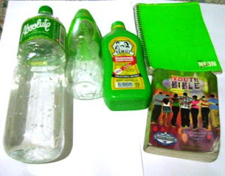
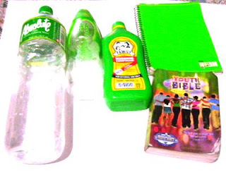
Image using RW algorithm and GW algorithm

Original Image


Image using RW algorithm and GW algorithm
Both images are better than the original image. I think that the image using RW algorithm is better in this case. The image using GW algorithm seems very bright and has poor contrast. This may be because the reference of for the GW algorithm is dependent on which RGB values are prominent in the image. This is due to the fact that the GW algorithm uses the mean of the RGB values of the image. For example if the color dominant in the image is green then the reference would be closer to the RGB values of the green. When we apply the GW algorithm on that image the green would appear closer to white. This explains why our image using the GW algorithm appeared brighter. If all the major hues are represented in the image then I think the GW algorithm would have better results since the average of the RGB values would most likely represent the average color of the world which is assumed to be gray.
I give myself a grade of 10 for this activity since I have done the algorithms and also included possible explanations for the results. Thank you for Billy Narag for helping me in this activity.
I give myself a grade of 10 for this activity since I have done the algorithms and also included possible explanations for the results. Thank you for Billy Narag for helping me in this activity.
Tuesday, August 26, 2008
A14 – Stereometry
Problem with using splin2d...Tried since the beginning of activity but failed...I guess 5 points for trying...
Subscribe to:
Posts (Atom)