A9 – Binary Operations

In this activity we want to estimate the area of one "cell" in the image that was given. A circle corresponds to one cell. What we want to do is to find the areas of all the circles then average them to get the approximate area of one circle. We do this by pixel counting following the procedure below.

1. Cut the given image to 256*256 sub-images. Save in filenames with increasing
index number, e.g. C1_01.jpg, C1_02.jpg etc.
2.Find it's thresholding value to separate the cells from the background.
3.Binarize the sub-images according to the threshold value using command imb2w.
4.Do opening and closing operations on the sub-images to clean the image (removing the isolated pixels, separating connected blobs and filling out holes). Opening operation is an erosion of an image followed by a dilation using the same structuring element. Closing is a dilation of an image followed by an erosion using the same structuring element.
4. Use bwlabel to label each contiguous blob on the binarized sub-images.
5. Find the areas of each blob by pixel counting and then find the estimate of the "cell" area using these values.

The image that I used is shown below as well as one of its sub-image.




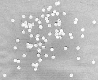
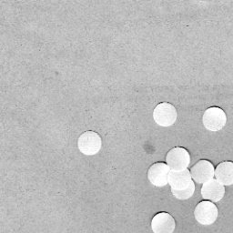
What I did was to first close the image using a 10 pixel radius circle then open it using the same circle. The result for the figure above is shown below.



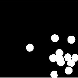
This is already a good image since it looks clean and there are no stray pixels. Although some of the blobs are still overlapping each other. We did this to all the sub-images and got the areas in each sub-images. This would be tiresome to do for 9 sub-images so I designed my program to do this automatically for each index. I plotted the histogram of the areas.



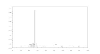
It looked like the areas are clustered between 400 and 600 so I looked more closely at that area and zoomed in. The image below is the histogram between 400 and 600.


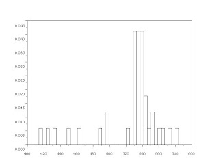
Looking carefully the correct range that should be considered must be from 480 to 580. So I took the average of the areas that fall between those values and get the standard deviation. The values calculated were area = 537.42857 and standard deviation = 18.544518. This is a fairly good estimate since the standard deviation is much smaller than the mean which means that the considered values are not that far from the real value of the area.

Thank you for Julie Mae Dado, Marge Maallo (Happy Birthday), Cole Fabros, Rafael Jaculbia, Eduardo David, Jorge Presto and Billy Narag for their help.

I rate myself 10 out of 10 since I have successfully estimated the value of the are for each blob and I think that I have done what is necessary to estimate it accurately. Also, I have figured out a way to process the sub-images automatically without running them one by one.
The code is shown below:

function [bin, recurrence] = histogram(image_matrix)
imsize = size(image_matrix)
bin = matrix(0:(max(image_matrix)),[(max(image_matrix)+1),1]);
recurrence = bin.*0;
for i = 1:imsize(1)
for j = 1:imsize(2)
recurrence(image_matrix(i, j) + 1) = recurrence(image_matrix(i, j) + 1) + 1;
end
end
endfunction

chdir('C:\Documents and Settings\Abraham\My Documents\AP186\A9');
counter=1;
area=[]
j=1;
for j= 1:9
a="c1_0"+string(j)+".jpg"; //opening each filename automatically
i=imread(a);
im=im2bw(i,.8);
e=imread('e.bmp');
r=dilate(im,e); //closing operation
r=erode(r,e);
r=erode(im,e); //opening operation
r=dilate(r,e);
[b,n]=bwlabel(r);
[x,y]=histogram(b);
x=x(2:max(b+1));
y=y(2:max(b+1));
g=1;
for k=counter:counter+n-1
area(k)=y(g);
g=g+1;
end
counter=counter+n;
end

scf(1);
histplot(length(area),area);

x=find(area<600>480);
scf(2)
histplot(length(x), area(x));
a=area(x);

a=sum(a)/length(x) //area
y=stdev(area(x)) //error